
You can read the original post here. The post is protected under Creative Commons Attribution 4.0 International License.
This post is an exposition to some of the background material and details of the linear Beltrami solver, which is an indispensable tool for my group of research. Interested readers can find relevant codes on Lui's computational geometry lab.
The references for this post are:
Elliptic Partial Differential Equations and Quasiconformal Mappings in the Plane (PMS-48). Kari Astala, Tadeusz Iwaniec & Gaven Martin.
Teichmuller mapping (T-map) and its applications to landmark matching registration. Lui Lok Ming, Lam Ka Chun, Yau Shing-Tung & Gu Xianfeng.
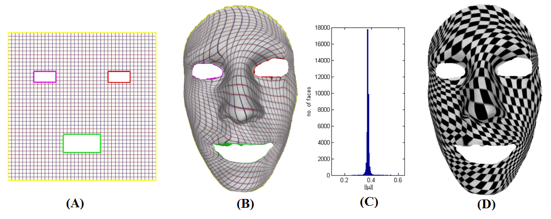
The method can be used to compute the surface quasiconformal homeomorphism such as this:
1.1. Measurable conformal structure
In one complex variable, holomorphicity is one of the most fundamental notions: suppose for simplicity we have a $ {\mathcal{C}^{1}}$ function $ {f=u+iv}$ defined on an open connected subset $ {\Omega}$ of $ {\mathbb{C}}$ (such is often called a domain). $ {f}$ is said to be holomorphic if its gradient satisfies the Cauchy-Riemann equations:
\[\displaystyle \begin{array}{rcl} Df(z)=\begin{bmatrix}u_{x} & u_{y}\\ v_{x} & v_{y} \end{bmatrix} & = & \begin{bmatrix}u_{x} & -v_{x}\\ v_{x} & u_{x} \end{bmatrix} \end{array} \]
where we have identified $ {\mathbb{C}}$ with $ {\mathbb{R}^{2}}$ in the usual manner. Note that the Jacobian \({J(f)=u_{x}^{2}+v_{x}^{2}\geq0}\) and by Sard's lemma the set of vanishing Jacobian is of measure zero. Thus as a mapping between planar domains, $ {f}$ is orientation preserving almost everywhere. Let's verify that $ {f}$ in fact preserve oriented angles on the infinitesimal level, where we define the action of $ {f}$ at a point $ {z_{0}\in\Omega}$ to be multiplication by the complex derivative
\[\displaystyle f'(z_{0})=\frac{\partial}{\partial z}f\big|_{z_{0}}=\frac{1}{2}\left(u_{x}+v_{y}\right)+\frac{i}{2}\left(u_{y}-v_{x}\right)=u_{x}-iv_{x}. \]
Recall that any complex number $ {a+ib}$ can be represented as
\[\displaystyle \begin{pmatrix}a & -b\\ b & a \end{pmatrix}. \]
(We used parenthese deliberately to distinguish representation of complex numbers from linear systems we consider). So this action is in effect applying the differential $ {df=\left(u_{x}+iv_{x}\right)dx+\left(u_{y}+iv_{y}\right)dy}$ to the vectors in the tangent plane at $ {z_{0}}$. Then that the action preserves angles follows immediately since the columns of the matrix are orthogonal, in the sense of Euclidean inner product. We can generalise the Euclidean inner product to other Riemannian metrics on $ {\Omega}$. Let $ {S(2)}$ denote the space of real-valued, symmetric, positive definite matrices with determinant one. Then a Riemannian metric on $ {\Omega}$ is defined as a mappping
\[\displaystyle A:\Omega\rightarrow\mathbb{R}_{>0}\cdot S(2). \]
\[\displaystyle A(z)=\begin{bmatrix}a & b\\ b & c \end{bmatrix} \]
This is the same as saying $ {A}$ is a symmetric positive definite $ {2}$-tensor field. On each tangent space at $ {z\in\Omega}$, the metric then defines an inner product
\[\displaystyle \langle\cdot,\cdot\rangle_{A}=\langle\cdot,A(z)\cdot\rangle. \]
We also say the Riemannian metric gives $ {\Omega}$ a Riemannian structure.
Remark 1 Typically, one talks about a Riemannian structure on a (real) smooth manifold, which is given by a smooth section of the $ {2}$-tensor bundle that is symmetric and positive definite, which is usually defined using charts. So strictly speaking, a Riemannian structure should come as an equivalence class of the metrics defined on these charts, which agree with each other whenerver the charts overlap. But here since $ {}$ has a global chart, there is seldom confusion.
It is clear from the definition of the metric $ {A}$ that it is conformally equivalent to another metric
\[\displaystyle G:\Omega\rightarrow S(2), \]
namely, $ {G=\left(\det A\right)^{-1/2}A}$. We say that $ {G}$ is bounded if the set $ {\{G(z):z\in\Omega\}}$ is bounded in $ {\mathbb{R}^{4}}$, and measurable if individual slots in the matrix are mesurable functions from $ {\Omega}$ to $ {\mathbb{R}}$.
Definition 1 (Mesurable conformal structure) If $ {G:\Omega\rightarrow S(2)}$ is bounded and measurable, we call $ {G}$ a measurable conformal structure on $ {\Omega}$. If $ {H:\Omega'\rightarrow S(2)}$ is a measurable conformal strucrture on $ {\Omega'}$, a homeomorphism $ {f:\Omega\rightarrow\Omega'}$ is said to be conformal from $ {\left(\Omega,G\right)}$ to $ {\left(\Omega',H\right)}$ if $ {f}$ preserves angles, i.e. for each $ {z\in\Omega}$, and vectors $ {\xi,\zeta}$ in the tangent plane at $ {z}$,
\[\displaystyle \langle f_{*}\xi,f_{*}\zeta\rangle_{H}=\phi\langle\xi,\zeta\rangle_{G} \ \ \ \ \ (1)\]
for some positive measurable function $ {\phi}$.
The conformal equivalence relation (1) can be translated to be a differential equation
\[\displaystyle D^{T}f(z)H(f(z))Df(z)=\phi(z)G(z), \]
where the derivative is interpreted in the weak sense. Note that taking determinants of both sides, we get $ {\phi(z)=J(z,f)}$, resulting the so-called Beltrami system
\[\displaystyle D^{T}f(z)H(f(z))Df(z)=J(z,f)G(z). \ \ \ \ \ (2)\]
Remark 2 If we take both $ {G=H=I}$, then we recover the usual conformal structure induced by the Euclidean metric. If $ {f=(u,v)}$ is conformal and differentiable, the equation (2) then reads
\[\displaystyle \begin{bmatrix}u_{x} & u_{y}\\ v_{x} & v_{y} \end{bmatrix}^{T}\begin{bmatrix}1 & 0\\ 0 & 1 \end{bmatrix}\begin{bmatrix}u_{x} & u_{y}\\ v_{x} & v_{y} \end{bmatrix}=\left(u_{x}v_{y}-u_{y}v_{x}\right). \]
When the Jacobian is non-singular, then after multiplying the inverse of $ {D^{T}f(z)}$ on both sides, we obtain the Cauchy-Riemann equation.
The solution to the equation (2) is of importance. For example, if $ {\Omega=\Omega'=\mathbb{D}}$, then the existence of the solution then implies all Riemannian metrics on $ {\mathbb{D}}$ are conformlly equivalent. This is in fact part of the uniformization theorem. Of course, for general different domains the solution may or may not exist, as can be seen from various ``conformal invariants'' for these domains. But for the moment we shall work only formally, to illustrate the ideas.
1.2. The linear distortion
Given a homeomorphism $ {f:\Omega\rightarrow\Omega'}$, we ask how far it deviates from a conformal map between standard conformal structures. The geometric observation is that conformal mappings map circles to circles, so we define
Definition 2 The linear distortion of $ {f}$ is
\[\displaystyle D(z,f)=\limsup_{r\rightarrow0}\frac{\max_{|\zeta|=r}|f(z+\zeta)-f(z)|}{\min_{|\zeta|=r}|f(z+\zeta)-f(z)|}. \]
First, we see that $ {f}$ is conformal at $ {z}$ if and only if $ {D(z,f)=1}$. If $ {f}$ is differentiable at $ {z}$, we can write the differential $ {df=f_{z}dz+f_{\bar{z}}d\bar{z}}$, where
\[\displaystyle \frac{\partial}{\partial z}f=\frac{1}{2}\left(u_{x}+v_{y}\right)+\frac{i}{2}\left(u_{y}-v_{x}\right);\quad\frac{\partial}{\partial\bar{z}}f=\frac{1}{2}\left(u_{x}-v_{y}\right)+\frac{i}{2}\left(u_{y}+v_{x}\right). \]
At the tangent space level, by triangle inequality we have
\[\displaystyle \left(|f_{z}|-|f_{\bar{z}}|\right)|dz|\leq|df|\leq\left(|f_{z}|+|f_{\bar{z}}|\right)|dz| \]
where both equalities can be obtained. So in this case we have
\[\displaystyle D(z,f)=\frac{|f_{z}|+|f_{\bar{z}}|}{|f_{z}|-|f_{\bar{z}}|}=\left(J(z,f)\right)^{-1}\left(|f_{z}|+|f_{\bar{z}}|\right)^{2},\]
since \({J(z,f)=|f_{z}|^{2}-|f_{\bar{z}}|^{2}}\). Thus if we take conformal structure on $ {\Omega'}$ to be the standard one $ {H=I}$, the Beltrami system (2) then reads
\[\displaystyle G_{f}(z)=\left(J(z,f)\right)^{-1}D^{T}f(z)Df(z)\]
whenever $ {J(z,f)>0}$. We call $ {G_{f}(z)}$ the distortion tensor of the mapping $ {f}$. Note that the operator norm of $ {G_{f}}$ is nothing but
\[\displaystyle \|G_{f}\|=D(z,f)=\left(J(z,f)\right)^{-1}\left(|f_{z}|+|f_{\bar{z}}|\right)^{2}\]
Assume the set of degeneracy Jacobian is of measure zero, we then have
\[\displaystyle G_{f}(z):\Omega\rightarrow S(2) \]
define a conformal structure on the domain $ {\Omega}$, where $ {f}$ is a conformal mapping from $ {(\Omega,G_{f})}$ to $ {(\Omega',I)}$.
1.3. Quasiconformal mappings and the Beltrami equation
Having only uniform control on the linear distortion does not guarantee the regularity of the mapping. This forces us to consider mappings in Sobolev spaces.
Definition 3 (Quasiconformal mapping) A homeomorphism $ {f:\Omega\rightarrow\Omega'}$ is called $ {K}$-quasiconformal if it is orientation-preserving, and $ {f\in W_{loc}^{1,2}(\Omega)}$, and the directional derivatives
\[\displaystyle \max_{\alpha}|\partial_{\alpha}f(z)|\leq K\min_{\alpha}|\partial_{\alpha}f(z)| \ \ \ \ \ (3)\]
for almost every $ {z\in\Omega}$.
Remark 3 Being merely a Sobolev function is not enough for a.e. differentiability, but only differentiable on lines a.e.. For this reason, in the above definition we had set
\[\displaystyle \partial_{\alpha}f(z)=\cos(\alpha)f_{x}(z)+\sin(\alpha)f_{y}(z) \]
for $ {\alpha\in[0,2\pi]}$. However, it is a theorem that if $ {f}$ is homeomorphic, then its derivative in in fact exists a.e.. So there is no trouble in the end.
The inequality (3) can be also formulated as
\[\displaystyle D(z,f)=\frac{|f_{z}|+|f_{\bar{z}}|}{|f_{z}|-|f_{\bar{z}}|}\leq K \]
for almost every $ {z\in\Omega}$. This means quasiconformal mappings map infinitesimal circles to ellipses. Rearranging the above inquality, we get
\[\displaystyle |f_{\bar{z}}(z)|\leq\frac{K-1}{K+1}|f_{z}(z)|. \]
Writing $ {\mu_{f}(z)=f_{\bar{z}}(z)/f_{z}(z)}$ when $ {f_{z}(z)\neq0}$ (which only happens on a measure zero set), we get $ {|\mu_{f}(z)|\leq\frac{K-1}{K+1}<1}$. Working backwards, we see that the equation
\[\displaystyle \frac{\partial f}{\partial\bar{z}}=\mu(z)\frac{\partial f}{\partial z} \ \ \ \ \ (4)\]
called the Beltrami euqation, where the Beltrami coeffiecient satisfies $ {\|\mu\|_{\infty}<1}$, is equivalent to the inequality (3). The existence of the solution (as a $ {K}$-quasiconformal homeomorphism) to the equation (4) when $ {\|\mu\|_{\infty}<1}$ is known as the measurable Riemann mapping theorem, and up to precomposition of comformal mappings is uniquely determined by $ {\mu:\Omega\rightarrow\Omega'}$. Let's convert (4) into matrix form. Write $ {\mu=\rho+i\tau}$. Separating the real and imaginary parts, we have
\[\displaystyle \begin{bmatrix}\rho-1 & \tau\\ \tau & -(\rho+1) \end{bmatrix}\begin{bmatrix}u_{x}\\ u_{y} \end{bmatrix}=\begin{bmatrix}\rho+1 & \tau\\ \tau & 1-\rho \end{bmatrix}\begin{bmatrix}-v_{y}\\ v_{x} \end{bmatrix}. \]
Since $ {\|\mu\|_{\infty}<1}$ , \({\det\begin{bmatrix}\rho+1 & \tau\\ \tau & 1-\rho \end{bmatrix}=1-\rho^{2}-\tau^{2}>0}\) for amoslt every \({z\in\Omega}\). Hence we see that
\[\displaystyle \begin{array}{rcl} \begin{bmatrix}-v_{y}\\ v_{x} \end{bmatrix} & = & \frac{1}{1-\rho^{2}-\tau^{2}}\begin{bmatrix}1-\rho & -\tau\\ -\tau & \rho+1 \end{bmatrix}\begin{bmatrix}\rho-1 & \tau\\ \tau & -(\rho+1) \end{bmatrix}\begin{bmatrix}u_{x}\\ u_{y} \end{bmatrix}. \end{array}\]
Denote $ {C=\begin{bmatrix}\rho-1 & \tau\\ \tau & -(\rho+1) \end{bmatrix}}$ and observe that it is symmetric. Then the above is
\[\displaystyle \begin{bmatrix}-v_{y}\\ v_{x} \end{bmatrix}=\frac{1}{1-\rho^{2}-\tau^{2}}C^{T}C\begin{bmatrix}u_{x}\\ u_{y} \end{bmatrix}.\]
Finally, denote \({-A=\frac{-1}{1-\rho^{2}-\tau^{2}}C^{T}C=\frac{-1}{1-\rho^{2}-\tau^{2}}\begin{bmatrix}-(1-\rho)^{2}-\tau^{2} & 2\tau\\ 2\tau & -\tau^{2}-(\rho+1)^{2} \end{bmatrix}}\) and it is easy to see that $ {A}$ is positive definite. Using the relation $ {v_{xy}=v_{yx}}$, we obtain a second order elliptic equation in divergence form:
\[\displaystyle -\nabla\cdot(A\nabla u)=0, \ \ \ \ \ (5)\]
where $ {\nabla\cdot(A\nabla)}$ is called the generalized Laplacian operator.
Remark 4 A solution $ {u}$ to the equation (5) can be used to determine $ {v}$ via the formula
\[\displaystyle \begin{bmatrix}-v_{y}\\ v_{x} \end{bmatrix}=-A \begin{bmatrix}u_{x}\\ u_{y} \end{bmatrix}. \]
And the function $ {f=u+iv}$ will thus be well defined, thanks to the integrable vector field condition $ {v_{xy}=v_{yx}}$.
Below the fold, we shall describe in details the discretisation of the Boundary value problem associated with the equation (5).
1.4. Discretisation and implementation
To simplify matters (and thus avoid discussion about impacts of "conformal invaraints") we assume $ {\Omega}$ is topologically a disk, and it is approximated by mesh, denoted $ {\mathcal{M}}$, with the following data structure called the indexed face set. Each vertex is indexed by a unique integer, and a face $ {F}$ of the mesh is stored as a triple $ {[i_{F_{1}},i_{F_{2}},i_{F_{3}}]}$ of the indices of its vertices. We shall also assmue $ {[i_{F_{1}},i_{F_{2}},i_{F_{3}}]}$ is oriented counterclockwisely. The data should look like those in the following table. In practice, the number of faces is about twice the number of vertices.
\[\begin{array} {cc} Vertex\ coordinates & Triangles \\ (g_{1},h_{1})& [i_{1},i_{2},i_{3}] \\ \cdots & \cdots \\ (g_V, h_V) & \cdots \\ & \cdots \\ & \cdots \\ & [i_{F_{1}},i_{F_{2}},i_{F_{3}}] \end{array}\]
In this discrete formulation, we shall compute the resulting mesh $ {\mathcal{M}'}$ after applying the discretized version of the generalized Laplacian. It suffices to know where the vertices go, that is a map between vertices
\[\displaystyle \begin{array}{rcl} v_{n}=(g_{n},h_{n}) & \mapsto & w_{n}=(s_{n},t_{n}). \end{array} \]
We extend on each face $ {T=[i_{T_{1}},i_{T_{2}},i_{T_{3}}]}$ linearly to get a simplicial mapping
\[\displaystyle f\big|_{T}(x,y)=\begin{bmatrix}u\big|_{T}(x,y)\\ v\big|_{T}(x,y) \end{bmatrix}=\begin{bmatrix}a_{T}x+b_{T}y+r_{T}\\ c_{T}x+d_{T}y+s_{T} \end{bmatrix}. \]
Then on each face we have the following approximation:
\[\displaystyle u_{x}\big|_{T}=a_{T};\quad u_{y}\big|_{T}=b_{T};\quad v_{x}\big|_{T}=c_{T};\quad v_{y}\big|_{T}=d_{T}. \]
Let's now calculate these from coordinates of the vertices of the faces $ {T}$ and $ {f(T)}$. It suffices to consider two edges of the triangle. Suppose $ {T}$ and $ {f(T)}$ have vertices $ {[v_{i},v_{j},v_{k}]}$ and $ {[w_{i},w_{j},w_{k}]}$ respectively. We consider the oriented edges $ {v_{j}-v_{i}}$ and $ {v_{k}-v_{i}}$ coinsident at $ {v_{i}}$. The simplicial mapping should map these edges to the corresponding oriented edges $ {w_{j}-w_{i}}$ and $ {w_{k}-w_{i}}$, i.e.
\[\displaystyle \begin{bmatrix}a_{T} & b_{T}\\ c_{T} & d_{T} \end{bmatrix}\begin{bmatrix}g_{j}-g_{i} & g_{k}-g_{i}\\ h_{j}-h_{i} & h_{k}-h_{i} \end{bmatrix}=\begin{bmatrix}s_{j}-s_{i} & s_{k}-s_{i}\\ t_{j}-t_{i} & t_{k}-t_{i} \end{bmatrix} \]
The determinant of $ {\begin{bmatrix}g_{j}-g_{i} & g_{k}-g_{i}\\ h_{j}-h_{i} & h_{k}-h_{i} \end{bmatrix}}$is just the signed area of the parallelogram, which is $ {2\cdot Area(T)}$. Note that we have chosen the same orientation for every $ {T}$ so the determinants calculated for each face are positive. Thus,
\[\displaystyle \begin{eqnarray*} \begin{bmatrix}a_{T} & b_{T}\\ c_{T} & d_{T}\end{bmatrix} & = & \frac{1}{2\cdot Area(T)} \begin{bmatrix}s_{j}-s_{i} & s_{k}-s_{i}\\ t_{j}-t_{i} & t_{k}-t_{i}\end{bmatrix} \begin{bmatrix}h_{k}-h_{i} & g_{i}-g_{k}\\ h_{i}-h_{j} & g_{j}-g_{i} \end{bmatrix} \\ & = & \begin{bmatrix}A_{T}^{i}s_{i}+A_{T}^{j}s_{j}+A_{T}^{k}s_{k} & B_{T}^{i}s_{i}+B_{T}^{j}s_{j}+B_{T}^{k}s_{k}\\ A_{T}^{i}t_{i}+A_{T}^{j}t_{j}+A_{T}^{k}t_{k} & B_{T}^{i}t_{i}+B_{T}^{j}t_{j}+B_{T}^{k}t_{k} \end{bmatrix}.\end{eqnarray*} \ \ \ \ \ (6)\]
where
\[\displaystyle A_{T}^{i}=\left(h_{j}-h_{k}\right)/2\cdot Area(T);\quad A_{T}^{j}=\left(h_{k}-h_{i}\right)/2\cdot Area(T);\quad A_{T}^{k}=\left(h_{i}-h_{j}\right)/2\cdot Area(T); \]
\[\displaystyle B_{T}^{i}=\left(g_{k}-g_{j}\right)/2\cdot Area(T);\quad B_{T}^{j}=\left(g_{i}-g_{k}\right)/2\cdot Area(T);\quad B_{T}^{k}=\left(g_{j}-g_{i}\right)/2\cdot Area(T). \]
The above gives in effect the discretisation of the gradient operator. The discretisation of the divergence operator is slightly more complicated. Here we want to take the diverence of a vector field defined on the faces, namely $ {(-d,c)_{T}}$, and the divergence is then a function of the vertices (roughly speaking, while gradient is applied on the graph, the divergence is applied on the dual graph). Since divergence measures the net flux across the boundary normalized by area, we define the divergence of any vector field $ {(X_{1},X_{2})_{T}}$ on faces to be
\[\displaystyle \text{Div}(X_{1},X_{2})(v_{i})=\sum_{T\in N_{i}}Area(T) \cdot A_{T}^{i}X_{1}(T)+Area(T) \cdot B_{T}^{i}X_{2}(T). \]
Here \(N_{i}\) denote the set of faces which contain the vertex indexed with \(i\). This is a right definition, since it is easy to check using (1) for each $ {v_{i}}$
\[\displaystyle \begin{array}{rcl} \text{Div}(-d,c)(v_{i}) & = & \sum_{T\in N_{i}}-Area(T) \cdot A_{T}^{i}d_{T}+Area(T) \cdot B_{T}^{i}c_{T}\\ & = & \sum_{T\in N_{1}}- Area(T) \cdot A_{T}^{i}\left( B_{T}^{i}t_{i}+ B_{T}^{j}t_{j}+B_{T}^{k}t_{k}\right)+\\ & & \quad\quad Area(T) \cdot B_{T}^{i}\left(A_{T}^{i}t_{i}+ A_{T}^{j}t_{j}+A_{T}^{k}t_{k}\right)\\ & = & 0. \end{array}\]
And similarly $ {\text{Div}(-b,a)(v_{i})=0}$. Finally, according to the equation (5), we have its discrete analog
\[\displaystyle \text{Div}\left\{ A \begin{bmatrix}B_{T}^{i}s_{i}+B_{T}^{j}s_{j}+B_{T}^{k}s_{k}\\ B_{T}^{i}t_{i}+B_{T}^{j}t_{j}+B_{T}^{k}t_{k} \end{bmatrix}\right\} =0\]
as a linear system in $ {s_{n}}$'s ready to solve (often in the least square sense).